Get Full Government Meeting Transcripts, Videos, & Alerts Forever!
Get email alerts on the Forecast Disaggregation Methods topic
No spam. Unsubscribe anytime.
PG&E, SCE and SDG&E outline distribution forecasting methods: feeder disaggregation, EV energy reconciliation and new AAFS handling
Summary
At the May 22 DFWG workshop, the three IOUs described how they disaggregate CEC IPR forecasts to feeders and service points. Key themes included starting from IPR vintages, using AMI and geospatial data for allocation, energy‑based reconciliation for EVs, and splitting AAFS shapes into summer/winter components where needed.
At the Distribution Forecasting Working Group workshop on May 22, PG&E, SCE and SDG&E described how they convert the CEC IPR system‑level forecast into circuit and feeder‑level forecasts used by distribution planners.
Why it matters: Distribution planning depends on circuit‑level forecasts of peak megawatts and hourly shapes. Differences in disaggregation methods — and in how utilities treat mobile loads such as EVs or emerging fuel‑substitution patterns — change where and when planners expect capacity needs.
PG&E (presentation by Mark Jimenez) described a multi‑step disaggregation starting from the 2023 IPR reliability forecast at the TAC level, then mapping that energy to the PG&E service footprint, using AMI and other customer data and a spatial simulation tool the utility calls “LOTS” to allocate growth across about 3,000 feeders. Jimenez said PV, storage and energy efficiency are handled with class‑based adoption potentials, propensity models and characteristic shapes. He emphasized EVs are modeled differently: "EV is different because the EV load can move around," he said, and PG&E applies an energy‑based adoption reconciliation that preserves the IPR energy while allocating hourly shapes to reflect where charging is expected.
On additional achievable fuel substitution (AAFS), Jimenez described a problem the utilities encountered with the 2023 IPR hourly files: the AAFS shape showed two distinct components with different seasonal growth rates (a winter heating component and a summer component). "The method that we choose to implement was to break the IPR shape into 2 different shapes in our forecast and apply different growth rates," Jimenez said, noting PG&E will refine that approach further in the next forecast cycle.
SCE (Lee Xu and Chris Mervarzi) explained a structure‑level disaggregation approach. Lee described a multivariable regression that combines SCADA, AMI, weather, economic and demographic data to produce structure‑level profiles, then allocates embedded growth from project workbooks and disaggregates remaining IPR growth. Chris detailed SCE’s DER allocation methods: residential PV and residential storage use historical adoption models to produce ZIP‑ and circuit‑level indicators; nonresidential DERs, energy efficiency and fuel substitution use allocation factors derived from billing‑system energy usage and third‑party building‑stock forecasts; EV (light‑duty) adoption was regressed against American Community Survey variables and median household income was the strongest predictor.
SDG&E (Waseem Al‑Safi and colleagues) described a process similar to the others, with specific inputs: historical DER adoption variables, local gas consumption for fuel substitution, and geospatial variables; SDG&E aggregates gas consumption to the circuit level (rather than ZIP code) for fuel‑substitution allocation. SDG&E also confirmed it uses an energy‑based approach for EVs and applies a pending‑loads bottoms‑up method for medium/heavy‑duty electrification this cycle.
Common issues discussed: all three utilities flagged EV forecasting as a key challenge because EV energy is mobile and peaks at specific charging sites (public DCFC can be highly peaky). Participants asked whether the utilities backtest feeder‑level simulations against realized installations; the utilities said they have limited backtesting to date and identified this as an area for improvement.
Bottom line: The three IOUs presented broadly similar high‑level workflows — start with an IPR vintage, adjust for local known loads, allocate by geospatial/propensity indicators and apply characteristic hourly shapes — but they differ in data sources, spatial granularity (ZIP vs circuit) and how they reconcile mobile loads and recent changes to AAFS hourly shapes.