Get Full Government Meeting Transcripts, Videos, & Alerts Forever!
Get email alerts on the Census Data Tools topic
No spam. Unsubscribe anytime.
Census webinar explains ‘65,000 rule’ and how to use data.census.gov to map PUMAs, MSAs and districts
Summary
U.S. Census Bureau trainers outlined differences between the Decennial Census and the American Community Survey, explained the ACS 65,000 population threshold for one‑year estimates, and demonstrated how to use data.census.gov filters to retrieve PUMAs, MSAs and congressional district data and downloads.
David Kraiker, a training specialist in the U.S. Census Bureau’s Data Dissemination and Training Branch, gave a livestreamed demonstration showing how to find and interpret data for larger census geographies and how to use data.census.gov.
Kraiker opened by distinguishing the Decennial Census — a 100% count pegged to April 1 of years ending in zero — from the American Community Survey (ACS), which samples monthly to produce demographic and socioeconomic characteristics. “The ten‑year census…is 100 percent data,” he said, and described the ACS as a continuous survey that uses a two‑month residency rule for inclusion.
A central takeaway was the Census Bureau’s 65,000‑person threshold for ACS reporting: geographies with populations over 65,000 qualify for one‑year ACS estimates; smaller areas receive five‑year pooled estimates. “Anything over, meaning anything…if it’s over 65,000 in population, you can get that data every year,” Kraiker said, noting one‑year tables typically appear in September while five‑year releases appear in December.
Kraiker reviewed the standard geography hierarchy (nation, state, county, tract, block) and highlighted commonly used large geographies — congressional districts, metropolitan and micropolitan statistical areas (MSAs), incorporated places and Public Use Microdata Areas (PUMAs). He explained that PUMAs are constructed from counties and tracts, typically contain 100,000 or more people, and are designed to enable more detailed ACS tabulation and microdata access.
Turning to data.census.gov, Kraiker walked attendees through a repeatable sequence: choose the reference year (he used 2024), select the survey (ACS one‑year or five‑year), pick the table or profile, then select the geography type (for example, PUMA or MSA) and the desired state/county. Using Essex County, New Jersey, as an example, he showed how to display PUMA maps, inspect profile tables (DP02, DP03, DP04) and toggle between map and table views.
Kraiker emphasized vintage differences and the importance of choosing the correct year: PUMA boundaries built on 2020 census data were reflected in a 2022 PUMA reconfiguration, producing different counts in his demonstration. He also showed how MSAs can change between vintages because Office of Management and Budget criteria incorporate commuting and economic data; he used New York–Newark and a pre‑2023 comparison to illustrate boundary changes.
For congressional districts, Kraiker demonstrated map layering to select a district and then use the “Within Other Geographies” tool to list census tracts fully or partially within that district (he highlighted Texas’s 35th Congressional District as an illustrative, elongated example). He advised GIS users to download ZIP files to obtain GEOID numbers for spatial joins.
In response to a question about urban/rural classifications, Kraiker said those definitions are distinct from the large‑geography constructs and are available on the platform but sometimes harder to locate; metropolitan and micropolitan areas are created using different (economic/commuting) criteria than simple urban/rural designations.
The session concluded with a reminder that the recording and supplemental materials will be posted to the Census Academy site within 30 business days and an invitation for attendees to complete the evaluation on exit.